reading-notes

Linear Regressions in Python

Readings

• How to Run Linear Regression in Python
• Linear Regressions in Python
• VIDEO: Introduction to Simple Linear Regressions

Reference

• Train and Test Splits
• What is Linear Regression

Notes

Linear Regression in Python

• Use Scikit-learn package
  • Package that simplifies the implementation of a wide range of Machine Learning methods for predictive data analysis, including linear regression
• What is a regression?
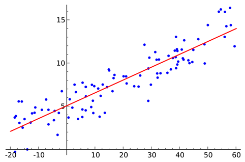
  • Finding the “line of best fit” through a scatter plot of data points

  

Key Regression Terms

• Best Fit – the straight line in a plot that minimizes the deviation between related scattered data points.
• Coefficient – also known as a parameter, is the factor a variable is multiplied by. In linear regression, a coefficient represents changes in a Response Variable (see below).
• Coefficient of Determination – the correlation coefficient denoted as 𝑅². Used to describe the precision or degree of fit in a regression.
• Correlation – the relationship between two variables in terms of quantifiable strength and degree, often referred to as the ‘degree of correlation’. Values range between -1.0 and 1.0.
• Dependent Feature – a variable denoted as y in the slope equation y=ax+b. Also known as an Output, or a Response.
• Estimated Regression Line – the straight line that best fits a set of scattered data points.
• Independent Feature – a variable denoted as x in the slope equation y=ax+b. Also known as an Input, or a predictor.
• Intercept – the location where the Slope intercepts the Y-axis denoted b in the slope equation y=ax+b.
• Least Squares – a method of estimating a Best Fit to data, by minimizing the sum of the squares of the differences between observed and estimated values.
• Mean – an average of a set of numbers, but in linear regression, Mean is modeled by a linear function.
• Ordinary Least Squares Regression (OLS) – more commonly known as Linear Regression.
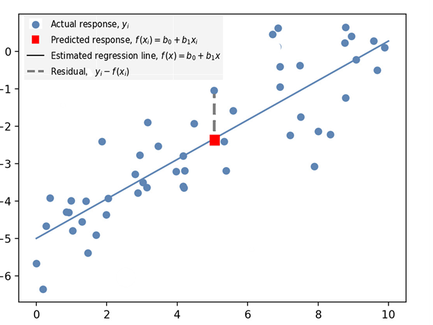
• Residual – vertical distance between a data point and the line of regression (see Residual in Figure 1 below).
• Regression – estimate of predictive change in a variable in relation to changes in other variables (see Predicted Response in Figure 1 below).
• Regression Model – the ideal formula for approximating a regression.
• Response Variables – includes both the Predicted Response (the value predicted by the regression) and the Actual Response, which is the actual value of the data point (see Figure 1 below).
• Slope – the steepness of a line of regression. Slope and Intercept can be used to define the linear relationship between two variables: y=ax+b.
• Simple Linear Regression – a linear regression that has a single independent variable.

Using Sci-learn

from sklearn.linear_model import LinearRegression
sklearn.linear_model.LinearRegression()

• Syntax and defaults
  • sklearn.linear_model.LinearRegression(fit_intercept=True, normalize=False, copy_X=True)
    • fit_interceptbool, default=True
      • Calculate the intercept for the model. If set to False, no intercept will be used in the calculation.
    • normalizebool, default=False
      • Converts an input value to a boolean.
    • copy_Xbool, default=True
      • Copies the X value. If True, X will be copied; else it may be overwritten.

Creating a Linear Regression

# Import the packages and classes needed in this example:
import numpy as np
from sklearn.linear_model import LinearRegression

# Create a numpy array of data:
x = np.array([6, 16, 26, 36, 46, 56]).reshape((-1, 1))
y = np.array([4, 23, 10, 12, 22, 35])

# Create an instance of a linear regression model and fit it to the data with the fit() function:
model = LinearRegression().fit(x, y) 

# The following section will get results by interpreting the created instance: 

# Obtain the coefficient of determination by calling the model with the score() function, then print the coefficient:
r_sq = model.score(x, y)
print('coefficient of determination:', r_sq)

# Print the Intercept:
print('intercept:', model.intercept_)

# Print the Slope:
print('slope:', model.coef_) 

# Predict a Response and print it:
y_pred = model.predict(x)
print('Predicted response:', y_pred, sep='\n')

How to Create a Linear Regression and Display it

# Import the packages and classes needed for this example:
import numpy as np
import matplotlib.pyplot as plt
from sklearn.linear_model import LinearRegression

# Create random data with numpy, and plot it with matplotlib:
rnstate = np.random.RandomState(1)
x = 10 * rnstate.rand(50)
y = 2 * x - 5 + rnstate.randn(50)
plt.scatter(x, y);
plt.show()

# Create a linear regression model based the positioning of the data and Intercept, and predict a Best Fit:
model = LinearRegression(fit_intercept=True)
model.fit(x[:, np.newaxis], y)
xfit = np.linspace(0, 10, 1000)
yfit = model.predict(xfit[:, np.newaxis])

# Plot the estimated linear regression line with matplotlib:
plt.scatter(x, y)
plt.plot(xfit, yfit);
plt.show()